How to use VLOOKUP() to find the closest match in Excel

One of Microsoft Excel’s most commonly used functions is VLOOKUP(). It’s a search function that lets you retrieve values by looking up a corresponding value. For instance, you might want to return the price of an item by using the item’s name or a student’s final grade by using the student’s name. It’s a flexible and extremely useful function. Most of the time you will want an exact match, but sometimes, you will need to return the closest matching value. In this article, you’ll learn about VLOOKUP() and then we’ll use it to find a match that almost matches the lookup value.

SEE: 83 Excel tips every user should master (TechRepublic)

I’m using Microsoft 365 on a Windows 10 64-bit system, but you can work with earlier versions. You can work with your own data or download the demonstration .xlsx and .xls files. This function works similarly in Excel for the web. This article assumes you have basic Excel skills such as entering functions and sorting, but even a beginner should be able to apply the instructions successfully.

How VLOOKUP() works in Excel

Excel’s VLOOKUP() function returns a corresponding value after matching a lookup value using the following syntax:

VLOOKUP(lookup_value, lookup_range, offset, is_sorted)

Table A explains these arguments. 

In a nutshell, VLOOKUP() uses a lookup value to return a value in another column. Now, let’s use it to find the closest matching value.

How to find the closest match with VLOOKUP()

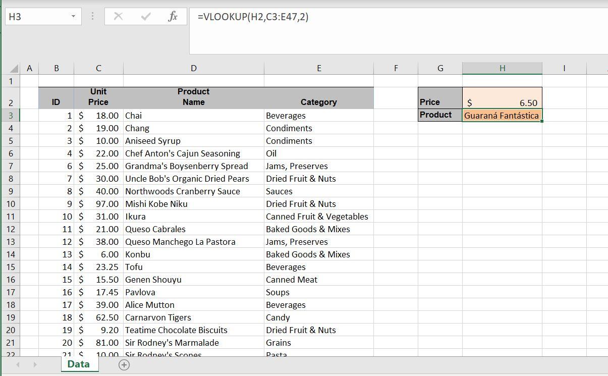
Most of the time you’ll use VLOOKUP() to find an exact match, but you can use it to find the closest match. You can use this technique when you’re unsure of the exact value or you must find a range of values. Now, let’s use this function to return a product name for a price, when the price isn’t an exact match using the data set shown in Figure A. The key is the input value in H2. Enter the value you’re trying to match, and the function in H3 returns the closest value it finds to the input value in H2. 

Figure A

Right now, the function in H3

=VLOOKUP(H2,C3:E47,2)

returns a value that doesn’t make sense—it’s wrong, but more about that in a minute. For now, let’s review how this function works within context. You’ll enter your guess price in H2. The function then uses this value to match a value in column C, the first column in the lookup range (but not necessarily the first column in the data set). When it doesn’t find an exact match, it stops looking when it finds the closest value to the value in H2 that’s less than that value and then returns the product name for the same row.

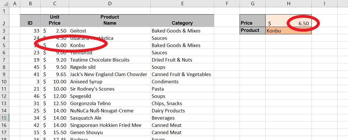
It’s not working because the data set isn’t sorted by the price column—the lookup value. Right now, the data set is sorted by the ID column. The fix is simple: run an ascending sort on the Unit Price column. To do so, click any cell inside the Unit Price column and choose Sort Smallest to Largest from the Sort & Filter dropdown in the Editing group on the Home tab. Or click AZ in the Sort & Filter group on the Data tab. Figure B shows the results. Using the function as is, the lookup column, in this case, the Unit Price column, must be sorted in ascending order.

Figure B

As you can see, VLOOKUP() returns the product Konbu, which has a price of $6. That price is the closest price to the lookup value in H2, 6.50, without being greater than 6.50. If you change the lookup value in H2 to 7 or 8.99, it continues to return Konbu. If you change the value in H2 to 9.10, it returns Tunnbröd.

SEE: Windows 10: Lists of vocal commands for speech recognition and dictation (free PDF) (TechRepublic)

At this point, you might be wondering what happens if you enter a value that’s an exact match. The function returns the product name for the exact match. If there are two matching values, it returns the first. This is how the VLOOKUP() works. What allows us to find a near match is the input value in H2. The technique doesn’t do anything special at all; I’ve simply exposed this behavior.

Remember that optional argument is_sorted? Right now, the function relies on the default value, TRUE. If you change that argument to FALSE, the function works only for exact matches in the Unit Price column, and it doesn’t matter if that column is sorted. However, it won’t work if the column is sorted in descending order.

This little-known behavior can be put to great use when exact values are unknown, and you need the flexibility to guess. 

Microsoft Weekly Newsletter

Be your company’s Microsoft insider by reading these Windows and Office tips, tricks, and cheat sheets.
Delivered Mondays and Wednesdays

Sign up today

Also see